Neural Form-Finding

The Problem

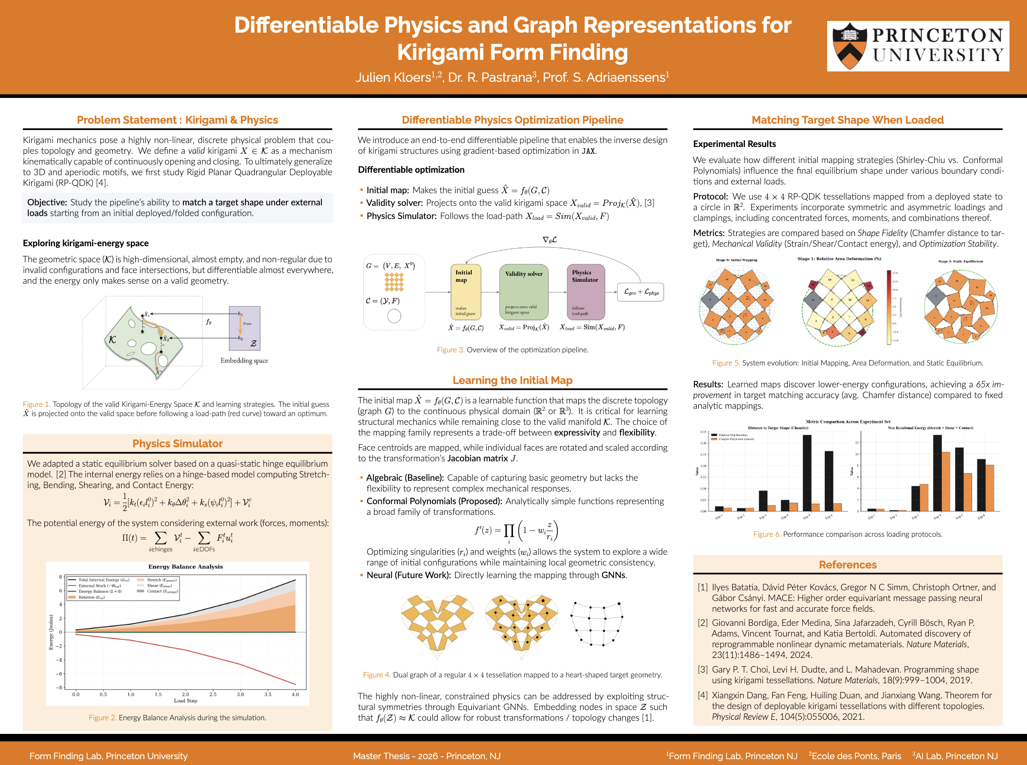
Kirigami — cut patterns in flat sheets that fold into three-dimensional deployable structures — is a beautiful design problem. I'm working specifically on rigid planar kirigami: structures where every tile is rigid, the whole thing has exactly one degree of freedom, and when fully closed, all voids completely disappear. Deployable, reversible, and geometrically precise.

The catch: the space of valid kirigami configurations is almost empty. Faces can't overlap. Tiles must stay connected. The deployability condition must hold globally. Deviate even slightly from a valid configuration and you almost certainly land outside the valid space. This makes the gradient landscape brutal for any optimization approach — which is exactly what makes it interesting.

The Approach

The entire pipeline is written in JAX. That's not incidental — differentiability and composability are the whole point, and JAX makes this natural.

Initial map. Rather than optimizing directly in the constrained valid space (a dead end), we learn an unconstrained function — the initial map — that proposes approximate kirigami geometries. It doesn't need to be valid. It just needs to be close.

Validity solver. The proposal is then projected onto the valid kirigami manifold, enforcing all geometric constraints: no overlaps, connected tiles, correct topology.

Physics simulator. Once we're in a valid configuration, we evaluate the mechanical response. The tiles are rigid — all energy lives in the hinges. Each hinge $h$ accumulates stretch, bending, and twist contributions:

where $\Delta\ell_h$, $\Delta\theta_h$, and $\Delta\phi_h$ are the elongation, bending angle, and twist deviations from the rest state.

Loss and backprop. The total loss combines a geometric term and the physical energy:

Gradients flow back through the physics, through the validity solver, through the initial map — one differentiable program, end to end.

@jax.jit
def forward(params, pattern):
    kirigami = initial_map(params, pattern)   # unconstrained proposal
    kirigami = validity_solver(kirigami)       # project to valid space
    energy   = physics_simulator(kirigami)     # hinge energies
    return geometric_loss(kirigami) + physical_loss(energy)

grad_fn = jax.value_and_grad(forward)

What's Next

The initial map was originally parameterized as complex polynomials. I'm currently replacing it with a GNN, which handles irregular topologies more naturally and should scale better across different cut patterns.

Beyond that, I'm exploring circle packing and Riemann map approximations as alternative representations of the valid kirigami space. The connection between conformal maps and the geometry of these structures is genuinely fascinating — and potentially a cleaner way to navigate the constraints. We'll see how far it goes before August.